When does Optimizer chooses FTS

When 

1)there is no INDEX exists
2)the table is small
3)the table has  high degree of parallelism
4)query uses full table scan hint
5)stats are stale
6)query requires most of the blocks
7)When implicit conversions takes place
8)When there are NULL's
9)query predicate does not use the leading edge of an index.


FTS uses larger IO calls.This means it read multiple blocks in an instance.
Making a fewer large I/O calls is cheaper than making many smaller calls.


High-water Mark 

This is a term used with table segments stored in the database. If you envision a table, for example, as a 'flat' structure or as a series of blocks laid one after the other in a line from left to right, the high-water mark (HWM) would be the rightmost block that ever contained data, as illustrated 

+---- high water mark of newly created table
|
V
+--------------------------------------------------------+
|  |  |  |  |  |  |  |  |  |  |  |  |  |  |  |  |  |  |  |
|  |  |  |  |  |  |  |  |  |  |  |  |  |  |  |  |  |  |  |
+--+--+--+--+--+--+--+--+--+--+--+--+--+--+--+--+--+--+--+

      high water mark after inserting 10,000 rows
                                    |
                                    v
+--------------------------------------------------------+
|x |x |x |x |x |x |x |x |x |x |x |x |  |  |  |  |  |  |  |
|x |x |x |x |x |x |x |x |x |x |x |x |  |  |  |  |  |  |  |
+--+--+--+--+--+--+--+--+--+--+--+--+--+--+--+--+--+--+--+


      high water mark after inserting 10,000 rows
                                    |
                                    v
+--------------------------------------------------------+
|x |x |x |x |x |x |x |  |  |  |  |  |  |  |  |  |  |  |  |
|x |x |x |x |x |x |x |  |  |  |  |  |  |  |  |  |  |  |  |
+--+--+--+--+--+--+--+--+--+--+--+--+--+--+--+--+--+--+--+

HWM starts at the first block of a newly created table. As data is placed into the table over time and more blocks get used, the HWM rises. If we delete some (or even all) of the rows in the table, we might have many blocks that no longer contain data, but they are still under the HWM, and they will remain under the HWM until the object is rebuilt, truncated, or shrunk (shrinking of a segment is a new Oracle 10g feature that is supported only if the segment is in an ASSM tablespace). 

The HWM is relevant since Oracle will scan all blocks under the HWM, even when they contain no data, during a full scan. This will impact the performance of a full scan,especially if most of the blocks under the HWM are empty. To see this, just create a table with 1,000,000 rows (or create any table with a large number of rows), and then execute a SELECT COUNT(*) from this table. Now, DELETE every row in it and you will find that the SELECT COUNT(*) takes just as long to count 0 rows as it did to count 1,000,000. This is because Oracle is busy reading all of the blocks below the HWM to see if they contain data. You should compare this to what happens if you used TRUNCATE on the table instead of deleting each individual row. TRUNCATE will reset the HWM of a table back to 'zero' and will truncate the associated indexes on the table as well. If you plan on deleting every row in a table, TRUNCATE;if it can be used it would be the method of choice for this reason. 

In an MSSM tablespace, segments have a definite HWM. In an ASSM tablespace, however, there is an HWM and a low HWM. In MSSM, when the HWM is advanced (e.g., as rows are inserted), all of the blocks are formatted and valid, and Oracle can read them safely. With ASSM, however, when the HWM is advanced Oracle doesn't format all of the blocks immediately they are only formatted and made safe to read upon their first use. So, when full scanning a segment, we have to know if the blocks to be read are 'safe' or unformatted (meaning they contain nothing of interest and we do not process them). To make it so that not every block in the table need go through this safe/not safe check, Oracle maintains a low HWM and a HWM. Oracle will full scan the table up to the HWM and for all of the blocks below the low HWM, it will just read and process them. For blocks between the 'low HWM' and the HWM, it must be more careful and refer to the ASSM bitmap information used to manage these blocks in order to see which of them it should read and which it should just ignore. 



MSSM-Manual Segment Space Management --Free space is maintained by Freelist
ASSM-Automatic Segment Space Management--Free Space is maintained by Bitmaps.

Dimensional Modeling Nomenclature

Normalization vs Denormalization

Normalization:

PROS:

• When writes are more than reads
• Vertically divided among columns i.e. split-ted into multiple tables.
• Updates and Inserts will be effective since no duplicates.
• Less use of heavy DISTINCT or GROUP BY queries since no duplicates.

CONS:

• JOINS due to multiple tables.
• Index strategies are not effective due to joins.

De-Normalization:

PROS:

• When reads are more than writes.
• SELECTS are very fast since we avoid JOINS and effective because of index strategies works very well with selective columns.

CONS:

• Updates and INSERTS becomes costly.

In real time , you should be good enough to choose the most read or most write tables to apply this concepts.

Unix Script to generate files based on unique values of a field

Below file has different mobile companies. I need to generate the files dynamically based on the unique values of the field.I can have blank values also.But I should not generate files for those.

Input:

Generate the Unique values :

Script to generate files based on the unique values. Here -z in the if condition represents the check for empty variable.

Output:

Remove Leading and Trailing spaces/tabs from each line in Unix using sed command

Input:








Command:

Output:

IMDB Datawarehouse

Resetting the ROW_NUMBER

What if I have the data like this?

RESET a RANK

SQL> select * from t1;

      DEPT DATE1
---------- ---------
       100 01-JAN-13
       100 02-JAN-13
       200 03-JAN-13
       100 04-JAN-13

select dept,  
       date1,
       rank () Over (partition by dept order by date1) rnk
from t1
order by date1;

      DEPT DATE1            RNK
---------- --------- ----------
       100 01-JAN-13          1
       100 02-JAN-13          2
       200 03-JAN-13          1
       100 04-JAN-13          3

The desired output is as follows. The last rnk=1 is becuase the Jan-04 record is the first record after the change.

      DEPT DATE1            RNK
---------- --------- ----------
       100 01-JAN-13          1
       100 02-JAN-13          2
       200 03-JAN-13          1
       100 04-JAN-13          1  <<<----------

Solution:

select dept, date1,
       CASE WHEN StartFlag = 0 THEN 1
            ELSE 1+StartFlag+NVL(lag(StartFlag) over (order by date1),0)
       END as rnk
from (select t1.*,
             (case when dept = lag(dept) over (order by date1)
                   then 1
                   else 0
              end) as StartFlag
      from t1
     ) t1
order by date1;

CUBE, ROLLUP , GROUPING SETS & GROUPING_ID

The GROUPING_ID function provides an alternate and more compact way to identify subtotal rows. Passing the dimension columns as arguments, it returns a number indicating the GROUP BY level.

Generate RANDOM values

You can generate random values from DBMS_RANDOM supplied package.

Get SAMPLE rows from a table

CUBE, ROLLUP and GROUPING SETS

GROUPING SETS simplifies the management of the subtotals

CUBE, ROLLUP and GROUPING SETS

CUBE:
Super aggregation is performed for each dimension.

CUBE, ROLLUP and GROUPING SETS

The CUBE, ROLLUP and GROUPING SETS functions are used in the GROUP BY clause to generate totals and subtotals.

ROLLUP can have more than one dimension, generating grand totals and subtotals:

Calculate maximum and minimum salary without using GROUP functions

Remove the extra spaces between the words in a sentence

Complex SQL Scenario

Get the deptno from employee table that are not in dept table and deptno from dept table that are not in employee table without using SET operators.

SELECT
COALESCE(DEPT.DEPTNO,EMP.DEPTNO)
FROM
EMP
FULL OUTER JOIN
DEPT
ON EMP.DEPTNO=DEPT.DEPTNO
WHERE EMPNO IS NULL OR DNAME IS NULL

/

Complex SQL Scenario

Get the minimum date if the consecutive code is same

CT KBB(DT DATE,COD VARCHAR(1))
INS INTO KBB VALUES('2014-01-01','A');
INS INTO KBB VALUES('2014-01-02','A');
INS INTO KBB VALUES('2014-01-03','D');
INS INTO KBB VALUES('2014-01-04','A');
INS INTO KBB VALUES('2014-01-05','D');
INS INTO KBB VALUES('2014-01-06','A');

Solution:

SEL EFF_DT,COD,

RANK() OVER(ORDER BY EFF_DT RESET WHEN COD<>MAX(COD) 

OVER(ORDER BY EFF_DT ROWS BETWEEN 1 PRECEDING AND 1 PRECEDING))

FROM KBB

Residual Condition in Explain Plan

Residual condition means a filter is applied on particular table to limit the number of rows fetched into Spool.
Say for example
Sel * from EMP where sal > 1000;

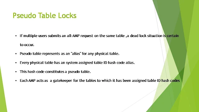
Pseudo Table in Explain Plan

It is a false lock which is applied on the table to prevent  two users from getting conflicting locks with all-AMP requests.
PE will determine an particular AMP to manage all AMP LOCK requests for given table and Put Pseudo lock on the table.

To put in Simple terms , its like an University with 10 gates and at a given time you can enter the university through one gate ( or main gate) for security check.

Reasons for product joins

1. Stale or no stats causing optimizer to use product join
2. Improper usage of aliases in the query.
3. missing where clause ( or Cartesian product join  1=1 )
4. non equality conditions like > ,< , between   example ( date)
5. few join conditions
6.  when or conditions are used.

last but not the least   product joins are not bad always!! sometimes PJ are better compared to other types of joins

Different types of skews

If you utilized unequally TD resources (CPU,AMP,IO,Disk and etc) this is called skew exists. Major are 3 types of skews (CPU skew, AMP/Data skew, IO Skew).

-Data skew?
When data is not distributed equally on all the AMPs.
-Cpu skew?
Who is taking/consuming more CPU called cpu skew.
-IO skew?
Who perform more IO Operation? Resulting in IO Skew

TENACITY and it's default value

• TENACITY specifies the amount of time in hours, to retry to obtain a loader slot or to establish all requested sessions to logon. 
• The default for Fast Load is “no tenacity”, meaning that it will not retry at all. 
• If several FastLoad jobs are executed at the same time, we recommend setting the TENACITY to 4, meaning that the system will continue trying to logon for the number of sessions requested for up to four hours.

Query to find the skew factor in Teradata

SELECT
TABLENAME,
SUM(CURRENTPERM) /(1024*1024) AS CURRENTPERM,
(100 - (AVG(CURRENTPERM)/MAX(CURRENTPERM)*100)) AS SKEWFACTOR
FROM
DBC.TABLESIZE
WHERE DATABASENAME= <DATABASENAME>
AND
TABLENAME =<TABLENAME>
GROUP BY 1;

Acceptable range for skew factor in a table

There is no particular range for skew factor.  In case of production systems, it is suggested to keep skew factor between 5-10.
There are various considerations for skew factor
- Number of AMPS
- Size of row in a table
- number of records in a table
- PI of a table
- Frequent access of table (Performance consideration)
- whether table getting loaded daily /monthly or how frequently data is being refreshed

How to skip the header row in the fastload script

RECORD 2; /* this skips first record in the source file */

Why Fload doesn’t support multiset table in Teradata?

Fload does not support Multiset table because of restart capability.

Say, the fastload job fails. Till the fastload failed, some number of rows was sent to the AMP's.

Now if you restart FLOAD,  it would start loading record from the last checkpoint and some of the consecutive rows are sent for the second time. These will be caught as duplicate rows are found after sorting of data.

This restart logic is the reason that Fastload will not load duplicate rows into a MULTISET table. It assumes they are duplicates because of this logic. Fastload support Multiset table but does not support the duplicate rows. Multiset tables are tables that allow duplicate rows. When Fastload finds the duplicate rows it discards it. Fast Load can load data into multiset table but will not load the duplicate rows

What are the types of HASH functions used in Teradata?

These are the types of HASH, HASHROW, HASHAMP and HASHBAKAMP. Their SQL functions are-

HASHROW (column(s))

HASHBUCKET (hashrow)

HASHAMP (hashbucket)

HASHBAKAMP (hashbucket)

To find the data distribution of a table based on PI, below query will be helpful. This query will give the number of records in each AMP for that particular table.

SELECT HASHAMP(HASHBUCKET(HASHROW(PI_COLUMN))),COUNT(*) FROM TABLENBAME GROUP BY 1.

How to create a table with an existing structure of another table with or without data and also with stats defined in Teradata?

CREATE TABLE new_TABLE AS old_TABLE WITH DATA;

CREATE TABLE new_TABLE AS old_TABLE WITH NO DATA;

CREATE TABLE new_TABLE AS old_TABLE WITH DATA AND STATS;

How to calculate the tablesize , database size and free space left in a database in teradata?

DBC.TABLESIZE and DBC.DISKSPACE are the systems tables used to find the space occupied.

Below Query gives the table size of each tables in the database and it will be useful to find the big tables in case of any space recovery.

SELECT         DATABASENAME,

TABLENAME,

SUM(CURRENTPERM/(1024*1024*1024)) AS "TABLE SIZE"

FROM

DBC.TABLESIZE

WHERE

DATABASENAME = 'DATABASE_NAME' AND TABLENAME = 'TABLE_NAME'

GROUP BY 1,2;

Below query gives the total space and free space available in a database.

SELECT

        DATABASENAME DATABASE_NAME,

        SUM(MAXPERM)/(1024*1024*1024) TOTAL_PERM_SPACE,

        SUM(CURRENTPERM)/(1024*1024*1024) CURRENT_PERM_SPACE,

        TOTAL_PERM_SPACE-CURRENT_PERM_SPACE as FREE_SPACE

 FROM

        DBC.DISKSPACE

 WHERE

        DATABASENAME = 'DATABASE_NAME'

group by 1;

Teradata Locks

Unix command to calculate the maximum length of a column in a file

I have a scenario where I have to find the maximum length of the data in a column in file.
Here, the column i need to find is for 12th column.



awk -F'|' 'NR>1{for (i=12; i<=12; i++) max[i]=(length($i)>max[i]?length($i):max[i])} END {for (i=12; i<=12; i++) printf "%d%s", max[i], (i==12?RS:FS)}' BETA.PAD.AUDIT.DAT

Find the maximum length of a line in a Unix file

awk ' { if ( length > L ) { L=length} }END{ print L}' <Filename>

Two MultiLoad Modes: IMPORT and DELETE

MultiLoad provides two types of operations via modes: IMPORT and DELETE. In MultiLoad
IMPORT mode, you have the freedom to "mix and match" up to twenty (20) INSERTs, UPDATEs or
DELETEs on up to five target tables. The execution of the DML statements is not mandatory for all
rows in a table. Instead, their execution hinges upon the conditions contained in the APPLY clause
of the script. Once again, MultiLoad demonstrates its user-friendly flexibility. For UPDATEs or
DELETEs to be successful in IMPORT mode, they must reference the Primary Index in the WHERE
clause.

The MultiLoad DELETE mode is used to perform a global (all AMP) delete on just one table. The
reason to use .BEGIN DELETE MLOAD is that it bypasses the Transient Journal (TJ) and can be
RESTARTed if an error causes it to terminate prior to finishing. When performing in DELETE mode,
the DELETE SQL statement cannot reference the Primary Index in the WHERE clause. This due to
the fact that a primary index access is to a specific AMP; this is a global operation.

The other factor that makes a DELETE mode operation so good is that it examines an entire block
of rows at a time. Once all the eligible rows have been removed, the block is written one time and a
checkpoint is written. So, if a restart is necessary, it simply starts deleting rows from the next block
without a checkpoint. This is a smart way to continue. Remember, when using the TJ all deleted
rows are put back into the table from the TJ as a rollback. A rollback can take longer to finish then
the delete. MultiLoad does not do a rollback; it does a restart.

Find the bad record in a file using Sed and AWK command

I have a file which has 23 million records loading into a stage table using Informatica.

Suddenly there is a failure due to bad record in between loading.Our file delimiter is " | " pipe. 

There is an extra pipe in between the fields. My file has 11 fields.

sed -n '14409589,2300000p' <filename>| awk -F "|" 'NF != 11'

returns the rows that have more than 11 columns.

Mixed Grain Fact Table

A mixed grain fact table is a fact table where we have measures with different grain. For example, one measure is weekly whereas the other measure is monthly. In this post I’d like to go through the advantages and disadvantages of that approach. The Kimball group clearly stated that measures in a fact table must have the same grain, see Kimball’s Toolkit book chapter 2.

As usual it is easier to explain “by example”:

It is a data mart. They have measures per week and per month, but they don’t have the measure on daily basis. Should we have 2 fact tables, one for weekly and one for monthly, like this: (1)

Or should we create a mixed grain fact table like this: (2)

In the above fact table, the black lines are weekly figures, whereas the red lines are monthly figures. They are both put in the same fact table, but on different measure columns. On the rows where the weekly measure exist, the monthly measure is zero. And vice versa. Therefore weekly and monthly total are correct:

select D.Week, sum(F.WeeklyMeasure) from FactMixedGrain F
join DimDate D on F.DimDate = D.DimDate group by D.Week

Result:

select D.Month, sum(F.MonthlyMeasure) from FactMixedGrain F
join DimDate D on F.DimDate = D.DimDate group by D.Month

Result:

Usually the main reason of doing option (2) is to have both the weekly and monthly measures in 1 fact table. This is done to save development effort, particularly ETL effort. It is easier to populate just 1 table than two tables.

That’s the advantage. Now the disadvantages. The issue with option (2) is that the grain of the fact table is mixed. There are 2 grains. In practice we have other dimension key columns in the fact table. And we also have other measure columns in the fact table. Some of these measures are weekly and some of them are monthly. Perhaps some of these measures are daily.

The issues with a fact table with a mixed grain like that are:

1. When the reporting from the table, we are risking mixing measures with different grains in the same formula, resulting in meaningless result.
2. The DateKey is used to indicate both the end of week and the end of month. This requires certain logic in the ETL, which prolong its development.
3. In the fact table we have black and red lines, indicating weekly and monthly grain. Black for weekly and red for monthly. We may end up having yellow lines too, for daily. And blue lines too, for quarterly. Oh, and green lines too, for yearly. After that, it will be very confusing. When we query the fact table, we wouldn’t be able to tell which line is which.
4. When we join this fact table with another fact table (drilling across), we are risking joining the wrong rows.

In option (2) above, the date dimension is used for 2 different grains in the fact table. Other examples like this are:

1. Product dimension used at the product group level and at the product category level.
2. Customer dimension used at the company level and at the group level.

When we have 2 or 3 dimensions, with each has dual grain like that, it becomes really confusing and risky.

In the above example, the same dimension key column has dual grain. In other cases, the mixed grain in the fact table is caused by different dimension key columns. One measure correspond to dim1, where as another measure correspond to dim2. Where measure1 has value, measure 2 is 0. And vice versa, like this:

And so it becomes really confusing. So I would recommend avoiding this design, mixing measures with different grains into the same fact table. Instead, it is better to put them into separate fact tables.

Complex SQL Scenario

Case1:Pick the max DATE1 if multiple distinct values.
Case2:If  no value or same value exists for DATE1 then pick maximum value from DATE2

SELECT
CLIENT_ID,
CASE 
WHEN COUNT(
DISTINCT  COALESCE(DATE1,TO_DATE('01-JAN-00','DD-MON-YY')))>1 
THEN MAX(DATE1) 
ELSE
MAX(DATE2)
END
FROM ADHOC
GROUP BY CLIENT_ID

Performance Tuning steps for Informatica Mapping

1. Reduce the number of transformations. There is always overhead involved in moving data between transformations.
2. Consider more shared memory for large number of transformations. Session shared memory between 12MB and 40MB should suffice.
3. Calculate once, use many times.

• Avoid calculating or testing the same value over and over.Calculate it once in an expression, and set a True/False flag.
• Within an expression, use variable ports to calculate a value than can be used multiple times within that transformation.
• Delete unnecessary links between transformations to minimize the amount of data moved, particularly in the Source Qualifier.
• This is also helpful for maintenance. If a transformation needs to be reconnected, it is best to only have necessary ports set as input and output to reconnect.
• In lookup transformations, change unused ports to be neither input nor output. This makes the transformations cleaner looking. It also makes the generated SQL override as small as possible, which cuts down on the amount  of cache necessary and thereby improves performance.
• The engine automatically converts compatible types.
• Sometimes data conversion is excessive. Data types are automatically converted when types are different between connected ports. Minimize data type changes between transformations by planning data flow prior to developing the mapping.
• Plan for reusable transformations upfront.
• Use variables. Use both mapping variables as well as ports that are variables.Variable ports are especially beneficial when they can be used to calculate a complex expression or perform a disconnected lookup call only once instead of multiple times
• Use mapplets to encapsulate multiple reusable transformations.
• Use mapplets to leverage the work of critical developers and minimize mistakes when performing similar functions.
• Reduce the number of non-essential records that are passed through the entire mapping.
• Use active transformations that reduce the number of records as early in the mapping as possible (i.e., placing filters, aggregators as close to source as possible).
• Select appropriate driving/master table while using joins. The table with the lesser number of rows should be the driving/master table for a faster join.
• Redesign mappings to utilize one Source Qualifier to populate multiple targets.This way the server reads this source only once. If you have different Source Qualifiers for the same source (e.g., one for delete and one for      update/insert), the server reads the source for each Source Qualifier.
• Remove or reduce field-level stored procedures.
• If you use field-level stored procedures, the PowerCenter server has to make a call to that stored procedure for every row, slowing performance.

4. Only connect what is used.
5. Watch the data types.
6. Facilitate reuse.
7. Only manipulate data that needs to be moved and transformed.
8. Utilize single-pass reads.
9. Sort the input data before passing to Joiner and Aggregate transformation.
10. In Lookup using customize query instead of default query. (Use '--' to overwrite lookup default order by clause).
11. Avoid using un-neccessary columns/port in sql query.
12. Filter un-neccessary data as closer to the source qualifier. (In case of Relational database include filter condition to the sql query).
13. In Joiner consider lesser value of data as Master Table.
14. In-case of mapping partition place aggregate transformation before the partition point.
15. Use Router instead of having multiple Filter transformations.

Generate date sequence given a range

SELECT TO_DATE('01-JUN-2015') + ROWNUM - 1
FROM (
  SELECT ROWNUM FROM (
    SELECT 1 FROM DUAL
    CONNECT BY LEVEL <= (
TO_DATE('01-JUL-2015') - TO_DATE('01-JUN-2015')
                                                  )
                                                  )
           );